dplyr wrangling for input to aqp

We take the raw data and process it for use in the aqp package.

We will use the magrittr “pipe” (%>%) operator to pipe or chain-together commands. The %>% facilitates passing variables to functions of the form f(x, y) as x %>% f(y). This is unnecessary with only a single “step,” but is particularly useful whenever you don’t want to create a bunch of intermediate variables or would like to keep the sequence of your workflow easy to read.

pocmaj <- pocmaj_raw %>%
  group_by(sample_id) %>%                 # group replicates together
  summarize(Ca = median(Ca), 
            Ti = median(Ti), 
            V  = median(V)) %>%           # calculate sample analyte median
  separate(sample_id, sep = " ",
           into = c("core", "depth")) %>% # split sample_id -> core + depth
  mutate(top = as.numeric(depth) * 100,   # calculate top and bottom depth
         bottom = top + 100)              #  (assuming 100 cm increments)

We group_by() sample_id and then summarize() the median() for each sample_id and analyte. This “flattens” a possible many-to-one relationship for values per depth. After that we separate() sample_id into core (site-level) and depth (layer-level) IDs using " " (a space) as the delimiter. Finally, we we scale depth by a factor of 100 to convert from meters to centimeters.

We could choose mean() and sd() as they are unbiased estimators for our layer-level summary function. The demonstration shown later that uses profile-level standard deviations in Vanadium value could be relatively easily modified to use layer-level variance derived from replicates/bulk/sub samples etc. Other summary statistics could be calculated such as max() for risk-assessment. We use median() because it is good for central tendency and we will be permuting the values around a “centroid” as our final demonstration.

Promote tbl_df to SoilProfileCollection via the formula interface

Once you have a site-level ID, top and bottom depth inside a data.frame-like object, you can use the formula interface to “promote” it to a SoilProfileCollection object. This provides user access to to site and layer-level fields via the site() and horizons() S4 methods, respectively.

For the sample data, or any stratified data without a bottom depth, we want to fill in a bottom depth using known sampling intervals and core geometry. This could be a bit of a “leap” if your values are actually “point” estimates and cannot be considered “representative” for the whole layer/block.

In aqp, the top and bottom depths are used as checks for depth-based ordering and topology – which some algorithms are sensitive to. depths<- sorts layer data (in @horizons slot) first on profile ID (core) then on top depth. From sorted layer data, the @site slot data are derived.

# promote pocmaj to SoilProfileCollection 
depths(pocmaj) <- core ~ top + bottom

core, top and bottom are all columns that exist in pocmaj. tbl_df and data.table are subclasses supported by the SoilProfileCollection in addition to data.frame.

depths(your.df) <- unique_site_ID ~ topdepth + bottomdepth

# plot soil profile sketch of one variable (V = Vanadium)
plot(pocmaj, color = "V", name = "hzID")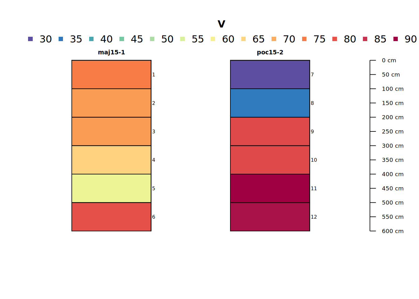

Producing site-level summaries from layer-level data with mutate_profile.

mutate_profile is a special variety of transform defined by the aqp package. It contains built-in iteration to support multiple non-standard evaluation expressions that are evaluated in the context of each single profile in a collection.

The result must either resolve to unit length for a profile (a site-level field) or equal in length to the number of layers for that profile (a layer-level field).

Let’s define a function that we can use to summarize SoilProfileCollection objects over arbitrary depth intervals.

#' Calculate site-level summary stats over interval [0, max.depth]
#' @name summarize_core
#' @param spc A SoilProfileCollection 
#' @param max.depth Vertical depth to truncate output to [0, max.depth]; default: 600;
#' @return A SoilProfileCollection
summarize_core <- function(spc, max.depth = 600) {
  
  # max.depth is subject to some basic constraints
  stopifnot(is.numeric(max.depth), length(max.depth) == 1, max.depth > 0)
  
  # truncate cores to a common depth interval [0, max.depth]
  res <- trunc(spc, 0, max.depth)  %>% 
    
    # for the depth-weighted mean, calculate horizon thickness
    #   identical to arithmetic mean if depth interval is constant
    transform(layer_wt = bottom - top) %>%
    
    # mutate_profile performs mutation by profile (site/core)
    mutate_profile(dwt_V = weighted.mean(V, layer_wt),
                   median_V = median(V), 
                   mean_V = mean(V), 
                   sd_V = sd(V))
  return(res)
}

# calculate depth-weighted average V within each core truncated to upper 200cm or 600cm
pocmaj2 <- summarize_core(pocmaj, 200)
pocmaj6 <- summarize_core(pocmaj, 600)

# create unique profile IDs
profile_id(pocmaj2) <- paste(profile_id(pocmaj2), "[0 - 2 m]")
profile_id(pocmaj6) <- paste(profile_id(pocmaj6), "[0 - 6 m]")

The below code demonstrates effects of total sampling depth on aggregation of stratified layers to “point” or site-level values.

# inspect result (a site-level field calculated from all layers)
pocmaj2and6 <- c(pocmaj2, pocmaj6)

# combined plot
plot(pocmaj2and6, color = "V", name = "hzID")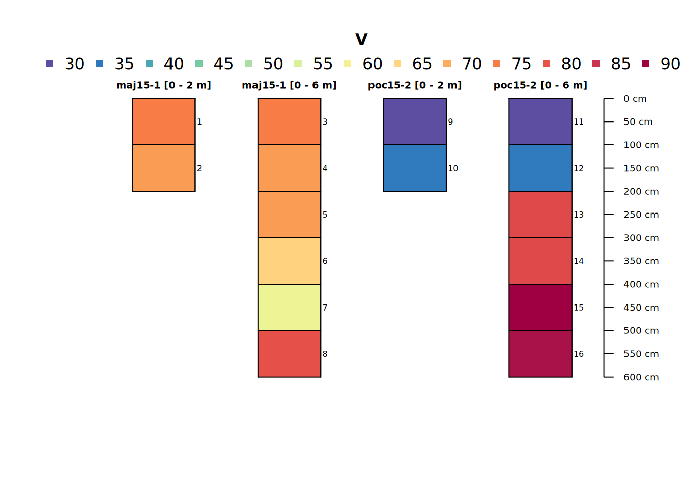

# inspect
site(pocmaj2and6)[,c(idname(pocmaj2and6), "dwt_V", "median_V", "mean_V", "sd_V")]

## # A tibble: 4 × 5
##   core              dwt_V median_V mean_V  sd_V
##   <chr>             <dbl>    <dbl>  <dbl> <dbl>
## 1 maj15-1 [0 - 2 m]  71.5     71.5   71.5  2.12
## 2 maj15-1 [0 - 6 m]  68.7     70     68.7  7.31
## 3 poc15-2 [0 - 2 m]  33.5     33.5   33.5  3.54
## 4 poc15-2 [0 - 6 m]  66.3     79     66.3 25.7

The summary statistics reflect what we noticed above in the profile plot and will be important later. One might be interested in aggregate properties of groups of cores summarized as above. We only have two unique cores – but that won’t stop us.

We can take this further and aggregate cores together into groups based on proximity, process, etc. This small two-site example dataset appears to have two different water bodies or areas where cores were collected. Presumably there are more data from there. In this case, we want to compare our 2-meter depth-truncated cores to the full 6-meter depth cores to test the effect of sampling depth on observed aggregate statistics. What are you missing by coring only to 2 rather than 6? To do this we will create a synthetic dataset.

Generating synthetic data

There is obviously natural variation in stratigraphy that is variably captured by a constant sampling interval. In addition, there are sampling errors such as uncertain datum, incomplete recovery and compaction. We will generate some realizations assuming that all layer boundaries have a standard deviation in depth of 10 centimeters and that V concentration varies related to the original value plus Gaussian noise related to a core-level variance parameter.

# assume variation in bottom depth amounts to a standard deviation of about 10% 1m core thickness
# i.e. that normal curve centered at the boundary between 100cm layers has SD of 10cm
horizons(pocmaj2and6)$layer_sd <- 10

To simulate we use the aqp method permute_profile. We use profileApply to iterate over cores, and aqp::combine to combine the 100 realizations we generate for each of the four input profiles.

# random number seed
set.seed(1234)

# iterate over cores, generate 100 realizations each, combine result
bigpocmaj <- aqp::combine(profileApply(pocmaj2and6, function(p) {
               # use a horizon-level field to produce geometric realizations
               pp <- perturb(p, boundary.attr = "layer_sd")
               
               # naive simulation of varying V values
               #  - core-specific standard deviation rounded base10 logarithm 
               #  - value cannot be negative [snaps to zero]
               pp$V <- pmax(0, pp$V + rnorm(nrow(pp), mean = 0, sd = 10^round(log10(pp$sd_V))))
               
               return(pp)
             }))

Note that this is a relatively naive way of simulating the property values, but also is perhaps reasonable considering the vertical granularity of observations in the Z dimension.

Inspecting the synthetic data

# simulated 400 realizations
#  4 profiles (2 cores, 0-2m and 0-6m case), 100 times each
length(bigpocmaj)

## [1] 400

# extract horizons tbl_df
h <- horizons(bigpocmaj)

# denormalize site-level core variable to horizon
h$core <- denormalize(bigpocmaj, "core")

# create factor levels for combined plots from multiple data sources
littlebig <- rbind(data.frame(pocmaj = "S", h[,horizonNames(pocmaj)]),
                   data.frame(pocmaj = "O",  horizons(pocmaj)))

# set up colors and labels
cbPalette <- c("#009E73", "#E69F00")
cbLabels <- c(sprintf("Median data & density (n = %s, bw = 5)", sum(!is.na(pocmaj$V))), 
              sprintf("Synthetic data (n = %s, bins = 100)", sum(!is.na(bigpocmaj$V))))

# plot
ggplot(littlebig, aes(x = V, after_stat(density),
                      color = factor(pocmaj), fill = factor(pocmaj))) + 
  geom_histogram(data = filter(littlebig, pocmaj == "S"), bins = 100) +
  geom_density(data = filter(littlebig, pocmaj == "O"), aes(x = V, fill = NULL), bw = 5) +
  geom_point(data = filter(littlebig, pocmaj == "O"), aes(x = V, y = 0)) +
  labs(title = "Median v.s. Synthetic bigpocmaj data\nVanadium by pXRF",
       x = "Vanadium (V), pXRF", y = "Density", color = "Legend", fill = "Legend") +
  scale_fill_manual(values = cbPalette, labels = cbLabels) +
  scale_color_manual(values = cbPalette, labels = cbLabels) +
  theme_bw()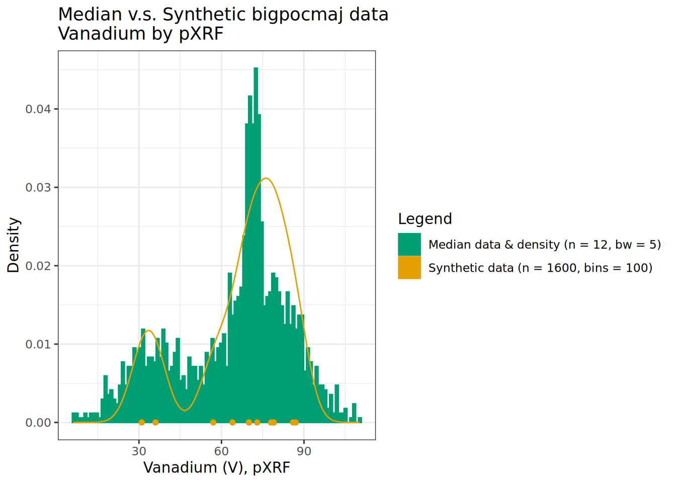

We see bi-modal patterns exhibited in the layer medians are reflected and fleshed out in our simulated data bigpocmaj. Notice the extreme values at edges of the empirical distribution – which are extrapolations beyond the range observed in the input data. The inclusion of the mixture of 2 and 6-meter deep profiles concentrates density in the range of distribution found in the upper depth portion of the profiles.

Grouped Profile Plot

This is a groupedProfilePlot() showing the different realizations generated from each of the four “parent” core descriptions. They look pretty noisy as they are unaware of any sort of meaningful pattern of depth covariance.

groupedProfilePlot(bigpocmaj[sample(1:length(bigpocmaj), size = 30),], 
                   groups = "core", color = "V", print.id = FALSE)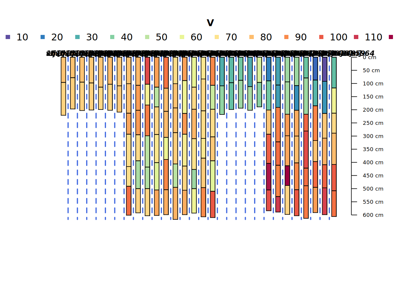

Compare percentiles

# raw v.s. median (analyte 1:1 with layer) v.s. synthetic
rbind(tibble(Source = "Raw",       Q = t(round(quantile(pocmaj_raw$V)))),
      tibble(Source = "Median",    Q = t(round(quantile(pocmaj2and6$V)))),
      tibble(Source = "Synthetic", Q = t(round(quantile(bigpocmaj$V)))))

## # A tibble: 3 × 2
##   Source    Q[,"0%"] [,"25%"] [,"50%"] [,"75%"] [,"100%"]
##   <chr>        <dbl>    <dbl>    <dbl>    <dbl>     <dbl>
## 1 Raw             29       62       73       82        95
## 2 Median          31       52       70       78        87
## 3 Synthetic        6       50       70       78       110

Note that the median()-based summary by layer “tamps” down the more extreme values from the raw data. However, the synthetic distribution captures the original range and then some. This is because we are “permuting” or “perturbing” Vanadium values using core-level variance parameters and assumptions of normality.

A maximum value of 110 pXRF is obtained in the synthetic sample – which is nearly 30 pXRF greater than the highest median, and about 20 pXRF greater than the highest observed raw value. For estimation of extrema rather than central tendency above approaches would need to be adjusted, but this is fine for this demonstration. It looks reasonably convincing when you compare to the density plot – though there really is just very little input data in this demo.

# use aqp::slab to calculate quantiles of V for 10cm "slabs" grouped by core
#  this is layer-level data result in a data.frame
hbpp <- slab(bigpocmaj, .oldID ~ V, slab.structure = 10)
hbpp <- hbpp[complete.cases(hbpp),]

# small jitter to prevent overplotting of medians
hbpp$p.q50 <- jitter(hbpp$p.q50, amount = 1)

# set up colors
cbPalette <- c("#009E73", "#E69F00", "#cc79a7", "#0072b2")

# plot
ggplot(hbpp, aes(x = V, y = top)) + 
       scale_y_reverse() +
       labs(title = "Synthetic `bigpocmaj` 10cm slab-wise median V [pXRF]\n w/ 0.05, 0.95 quantiles", 
            x = "Vanadium (V), pXRF", y = "Depth, cm", color = "Legend") +
       geom_path(data = hbpp, aes(x = p.q50, y = top, color = factor(.oldID)), linetype = 2) +
       geom_path(data = hbpp, aes(x = p.q5, y = top, color = factor(.oldID)), linetype = 3) + 
       geom_path(data = hbpp, aes(x = p.q95, y = top, color = factor(.oldID)), linetype = 3) + 
       scale_color_manual(values = cbPalette) +
       theme_bw()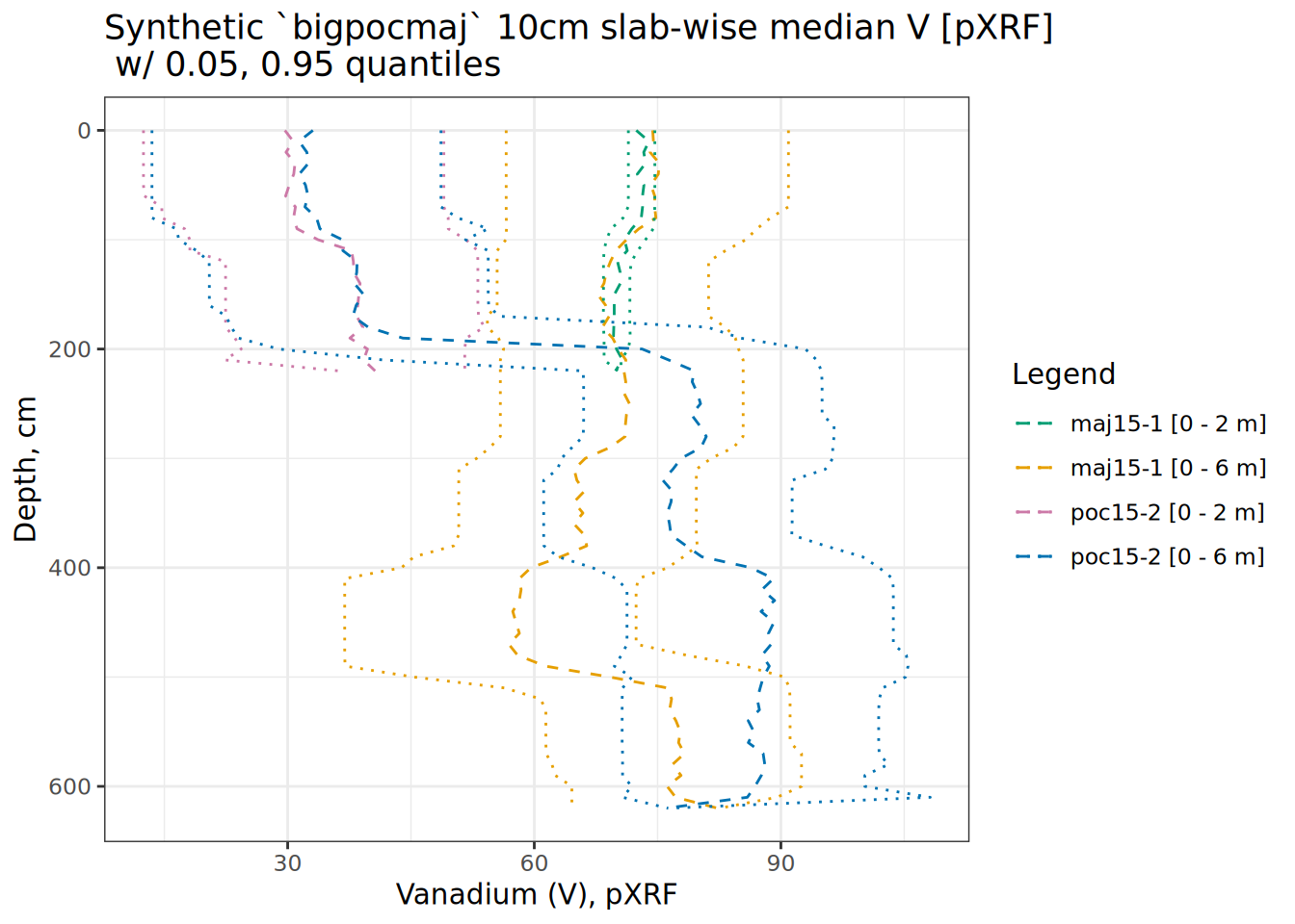

# calculate site-level summary stats for each simulated core
simulated.groups <- summarize_core(bigpocmaj, 600) %>% 
  
  # group by "core" (original profile ID)
  aqp::groupSPC(core) %>%
  
  # summarize profile stats by original core group
  aqp::summarizeSPC(mean_dwt_V = mean(dwt_V), 
                    mean_median_V = mean(median_V), 
                    mean_mean_V = mean(mean_V), 
                    mean_sd_V = mean(sd_V),
                    sd_dwt_V = sd(dwt_V), 
                    sd_median_V = sd(median_V), 
                    sd_mean_V = sd(mean_V), 
                    sd_sd_V = sd(sd_V))

## converting core to factor

# inspect
head(simulated.groups)

## # A tibble: 6 × 9
##   core       mean_dwt_V mean_median_V mean_mean_V mean_sd_V sd_dwt_V sd_median_V
##   <chr>           <dbl>         <dbl>       <dbl>     <dbl>    <dbl>       <dbl>
## 1 maj15-1 […       71.9          72.1        72.1      1.97       NA          NA
## 2 maj15-1 […       72.0          71.9        71.9      1.76       NA          NA
## 3 maj15-1 […       72.2          72.0        72.0      1.80       NA          NA
## 4 maj15-1 […       72.6          73.0        73.0      2.64       NA          NA
## 5 maj15-1 […       71.1          71.0        71.0      2.93       NA          NA
## 6 maj15-1 […       71.6          71.5        71.5      2.70       NA          NA
## # ℹ 2 more variables: sd_mean_V <dbl>, sd_sd_V <dbl>

So, we may not completely believe the values coming out of this naive simulation, but it shows the workflow for how you would summarize a larger amount of data.

Also possibly gives some ideas on how to begin comparing observed data to synthetic data. The output generally reflects the pattern we saw from the individual cores – with a little more fuzziness.

Commentary

The analysis shown above can be useful for demonstrating sensitivity to factors that affect scaling and aggregation of depth-dependent properties. In these lake cores factors could include: the depth range sampled, core recovery/compaction/fall-in, variation in analytes compared to “random noise” around a single centroid, use of individual v.s. group v.s. global variance parameters, and more.

We assume standard deviations for core depth ranges are constant at 10 cm / 10% of a 1-meter slice. This produces a slight perturbation to the parent geometry without dramatically influencing the overall degree of aggregation. We further assume that the variation in the analyte can be “perturbed” for a layer based on the original value for that layer plus a Gaussian offset related to the whole-core variation in analyte.

With the above assumptions it is tacitly accepted that there is a single “mode” within a core – clearly this is not always the case in nature, especially as depth increases – but the question of whether nature can be approximated by a single mode will perennially be an interesting one. The above analysis is suggestive of two or more distinct modes of V value in layers: those with value ~70 pXRF, and those with about half that – but that is just based on two unrelated cores.

Ideally, simulation parameters would be based on more than one core and would be depth-dependent.

permute_profile only deals in Gaussian offsets of boundaries which means it is limited for generating profiles that exhibit more “natural” depth-skewed distributions or long-range-order types of variation in space. That means you shouldn’t expect it to be able to generate the stuff that you might find in nature – you have to sample that yourself! And then permute it :)! That said, in the future permute_profile will likely be expanded to support additional distributions, parameters, models or covariance structures that can be derived from experimental/observed data.

Next steps

If you enjoyed this tutorial and want to expand on what you worked on here, you could try modifying the code to explore Calcium (Ca) or Titanium (Ti) values instead of Vanadium (V). Dewey’s tutorial where this dataset came from has tips on using facets to plot multiple analytes etc. Also you can adjust the layer boundary standard deviation size or number of realizations (currently 100) per profile. You could also try and load your own datasets into this routine and modify it for your own use. I will caution you about naive assumptions of normality and independence one last time, though.

If discussion about identification of similar layers within depth-stratified data intrigues you, functions in aqp such as generalize_hz, hzTransitionProbabilies, genhzTableToAdjMat and mostLikelyHzSequence may be useful. Identifying “depth modes” in soils data is essential to properly categorizing knowledge and generating accurate interpretations of properties. Dylan Beaudette has developed several routines for visualizing generalized horizon patterns such as plotSoilRelationGraph and plots that show simultaneous horizon transition probabilities for multiple generalized horizons across depth.

Here is a tutorial on initial steps for developing generalized horizon concepts for the Statistics for Soil Survey course. It needs to be expanded to demonstrate some of the graphical and modeling components.

The stratigraphic diagrams with tidypaleo & ggplot2 tutorial from Dewey has some great paleolimnology-depth-dendrograms that are getting at the same fundamental “depth mode” concepts – this might be worth exploring especially in the context of aqp::slice and aqp::slab. It also would be helpful if you are interested in expanding the plots in this tutorial to show multiple analytes.