{ggspc}

The goal of {ggspc} is to provide custom ‘Stat’, ‘Geom’ and ‘theme’ definitions for ‘SoilProfileCollection’ object compatibility with ‘ggplot2’.

Installation

You can install the development version of {ggspc} like so:

remotes::install_github("brownag/ggspc")

Example

This a example shows how to solve the common problem of plotting variables contained in a SoilProfileCollection with ggplot2::ggplot()

library(aqp)
#> The legacy packages maptools, rgdal, and rgeos, underpinning the sp package,
#> which was just loaded, will retire in October 2023.
#> Please refer to R-spatial evolution reports for details, especially
#> https://r-spatial.org/r/2023/05/15/evolution4.html.
#> It may be desirable to make the sf package available;
#> package maintainers should consider adding sf to Suggests:.
#> The sp package is now running under evolution status 2
#>      (status 2 uses the sf package in place of rgdal)
#> This is aqp 2.0
library(ggspc)
library(ggplot2)

data(loafercreek, package = "soilDB")
GHL(loafercreek) <- "genhz"

Basics

This is a demonstration of what is possible with a simple fortify(<SPC>) method defined. The “fortify” method makes it such that names from horizon and site slots of the SPC can be used in ggplot() aesthetics via aes().

# site v.s. site level
ggplot(loafercreek, aes(earthcovkind1, slope_field)) +
  geom_boxplot(na.rm = TRUE)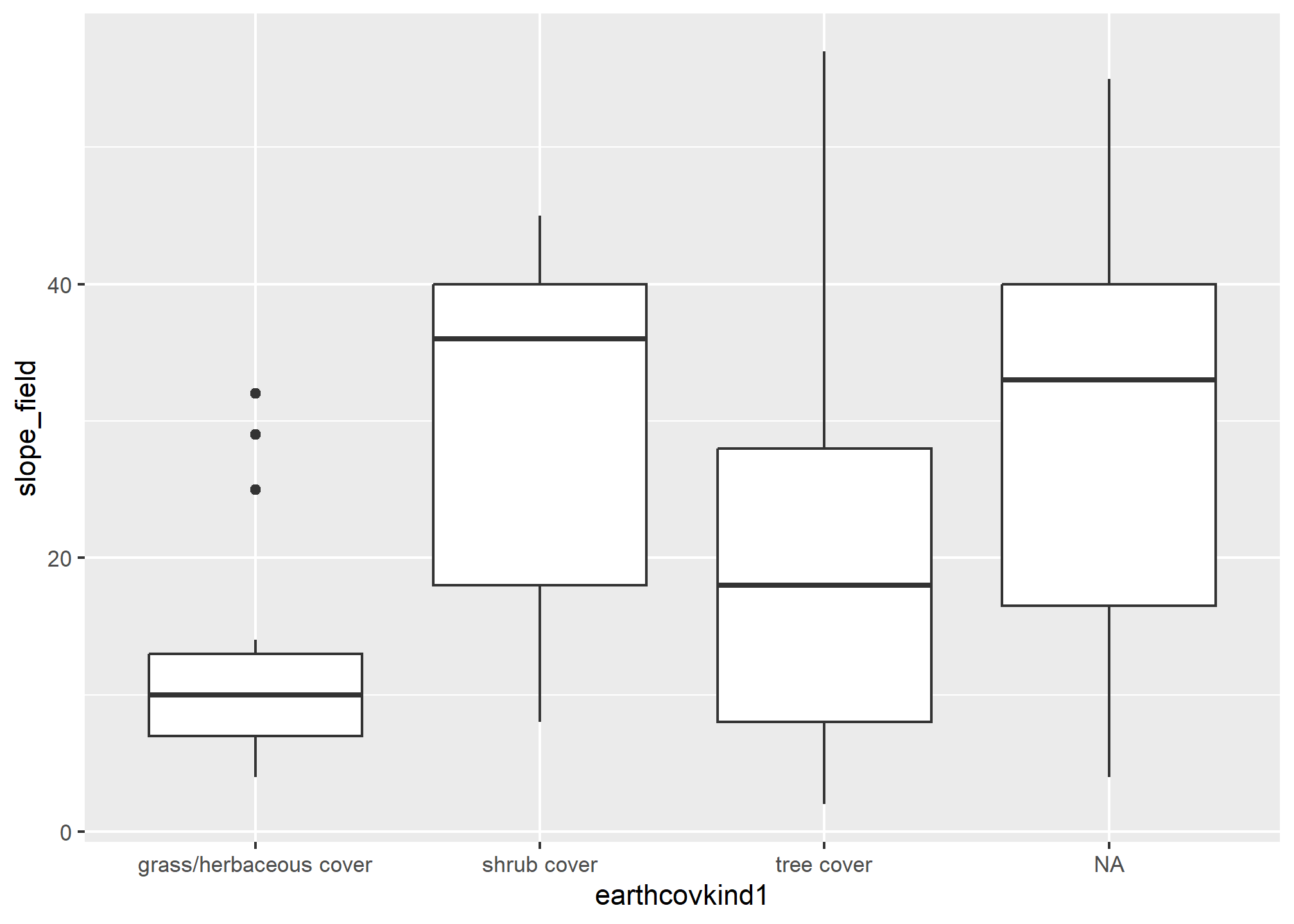

# site v.s. horizon level
ggplot(loafercreek, aes(hillslopeprof, clay)) +
  geom_boxplot(na.rm = TRUE)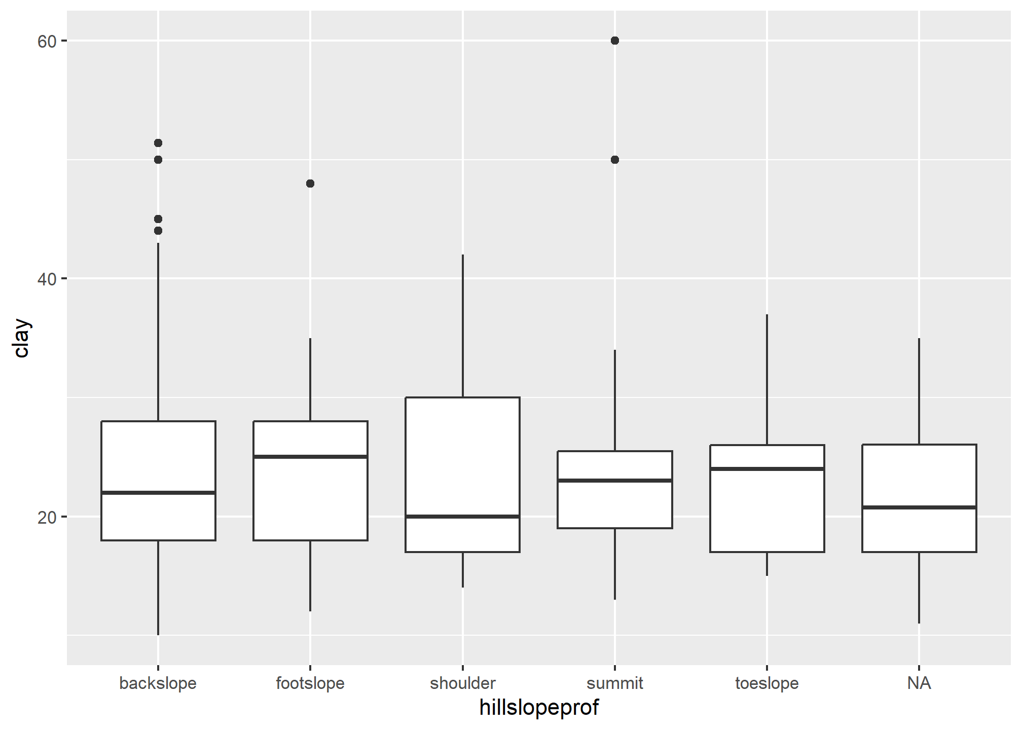

# horizon v.s. horizon level
ggplot(loafercreek, aes(clay, genhz)) +
  geom_boxplot(na.rm = TRUE)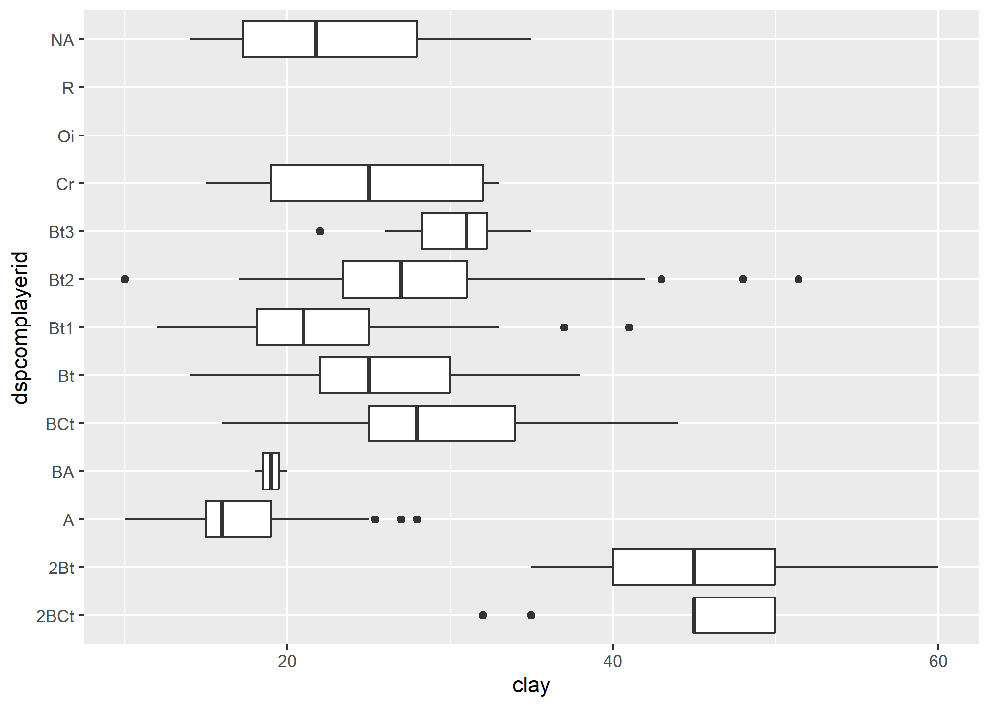

Depth Weighted Aggregation (stat_depth_weighted())

The stat_depth_weighted() function is a specialized {ggplot2} statistic intended for calculation of depth-weighted values for horizon data in a SoilProfileCollection. The default uses a constant interval from=0 to=200 (centimeters), but the intervals of interest may alternately be specified as site-level column names (unquoted), and therefore may vary between profiles.

Currently, stat_depth_weighted() only supports the “point” geometry type, but in future “boxplot” and others may be supported.

# default y aesthetic is the profile_id(<SPC>)
ggplot(loafercreek[1:10], aes(clay)) +
  stat_depth_weighted(na.rm = TRUE)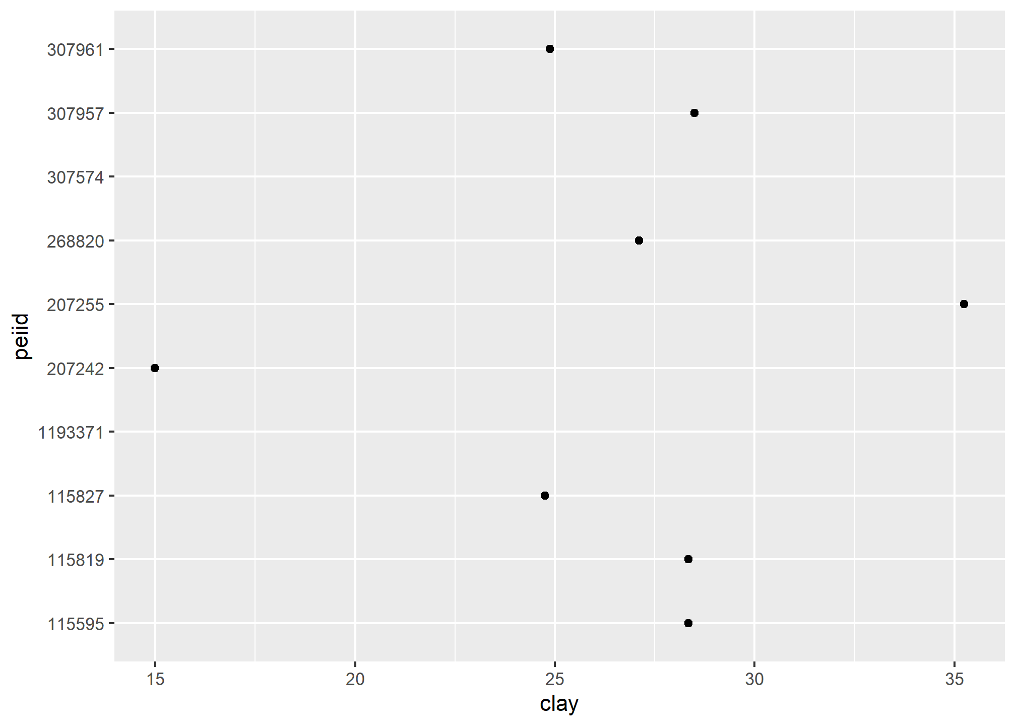

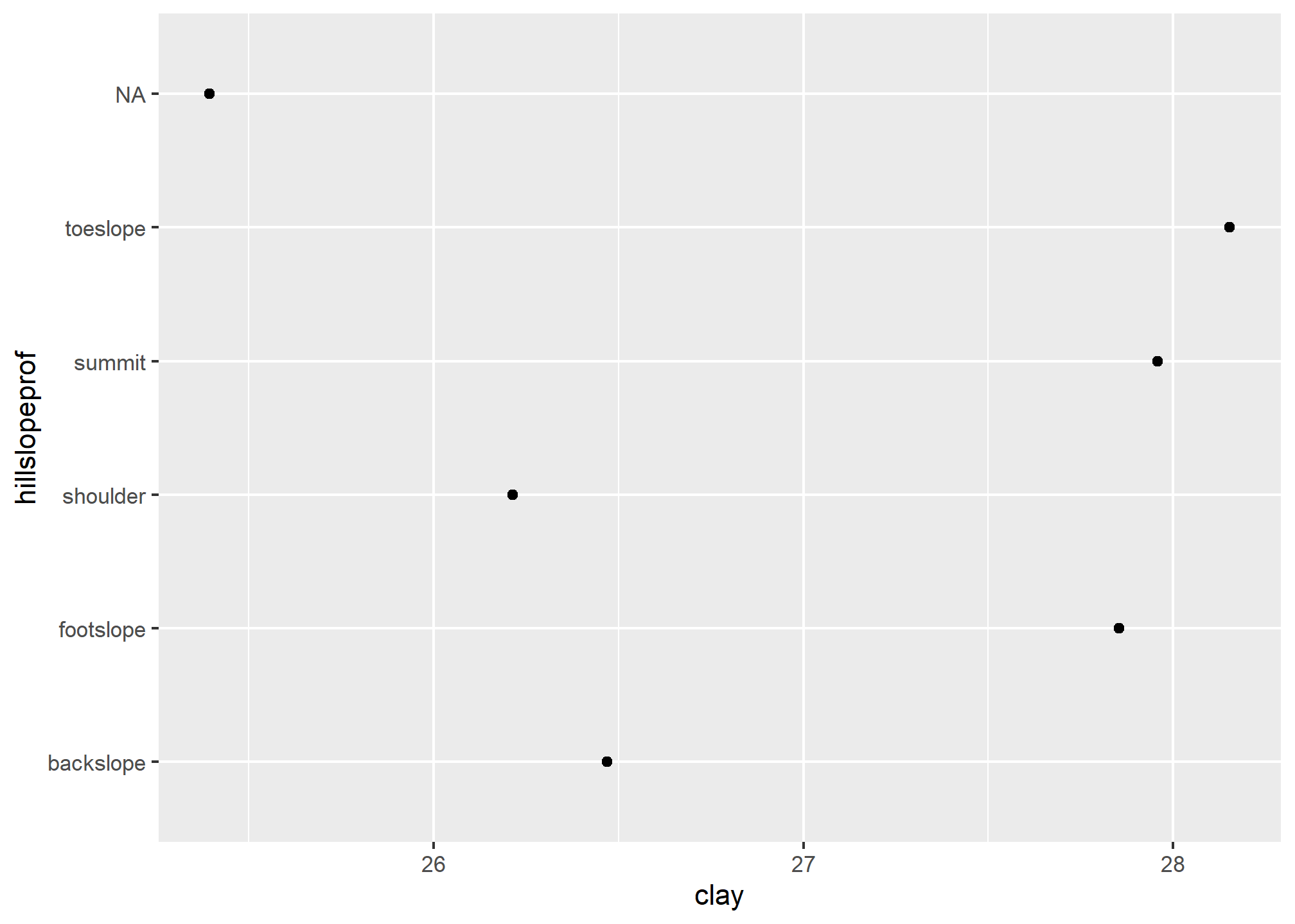
# can use alternate y aesthetic, e.g. hillslopeprof
ggplot(loafercreek, aes(clay, hillslopeprof)) +
  stat_depth_weighted(na.rm = TRUE)

# continuous y axes works too (horizon v.s. horizon)
ggplot(loafercreek, aes(clay, sand)) +
  stat_depth_weighted(na.rm = TRUE)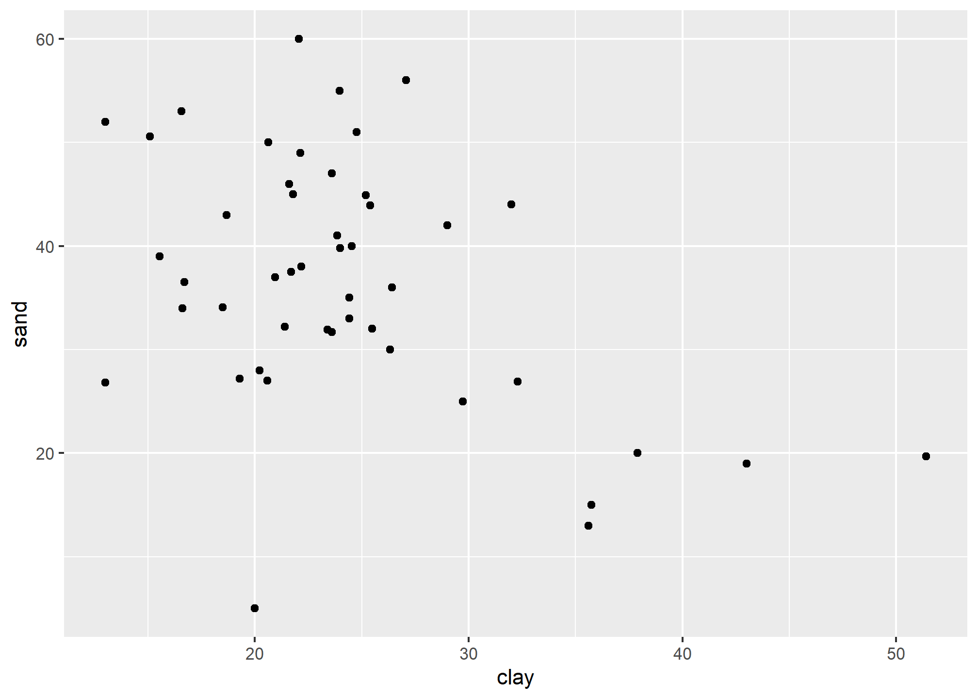

# continuous y (horizon v.s. site)
ggplot(loafercreek, aes(clay, slope_field)) +
  stat_depth_weighted(na.rm = TRUE)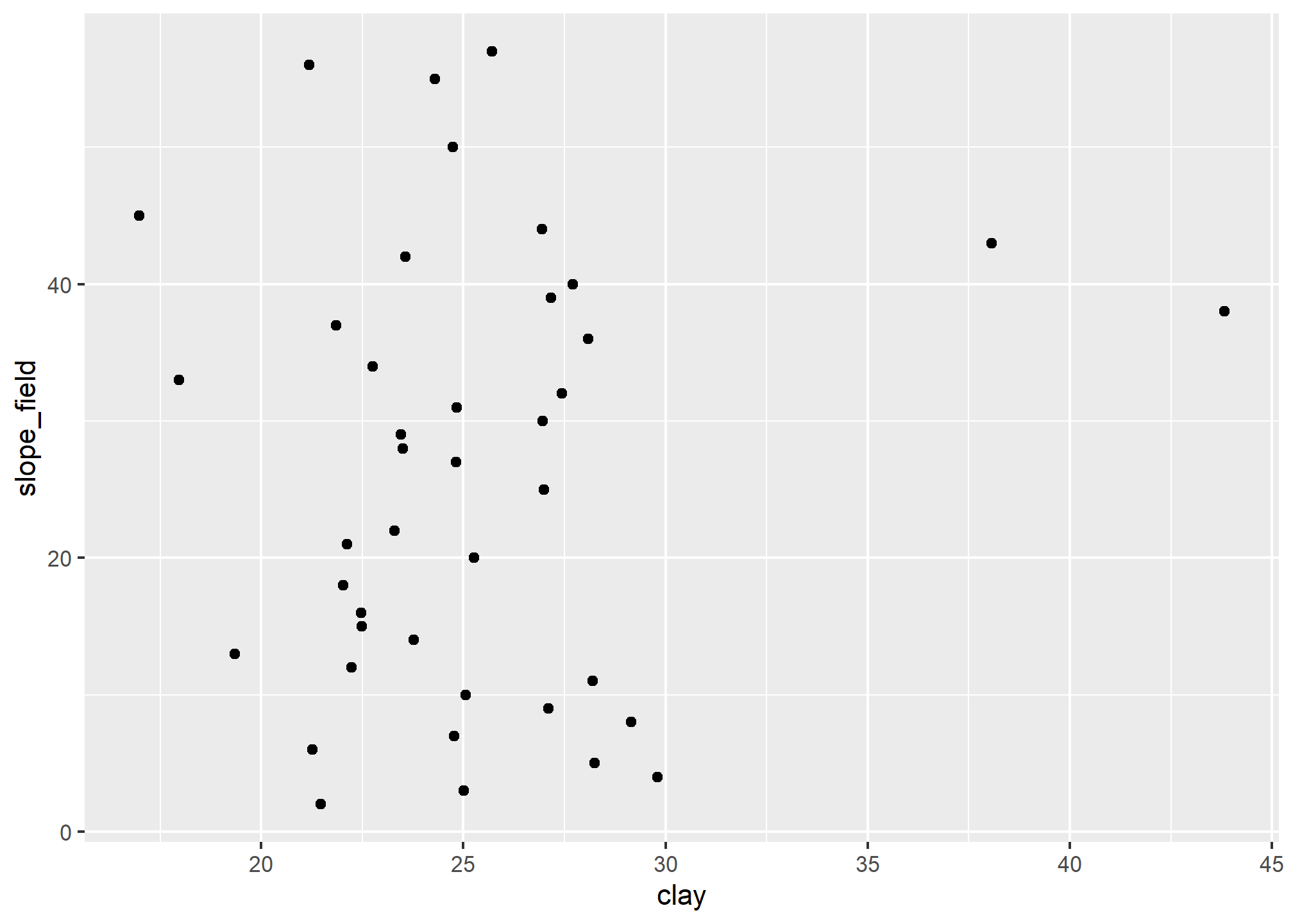

# can combine with typical ggplot geoms (0-200cm mean over boxplots)
ggplot(loafercreek, aes(clay, hillslopeprof)) +
  geom_boxplot(na.rm = TRUE) + 
  stat_depth_weighted(na.rm = TRUE, col = "red", pch = 17, cex = 3)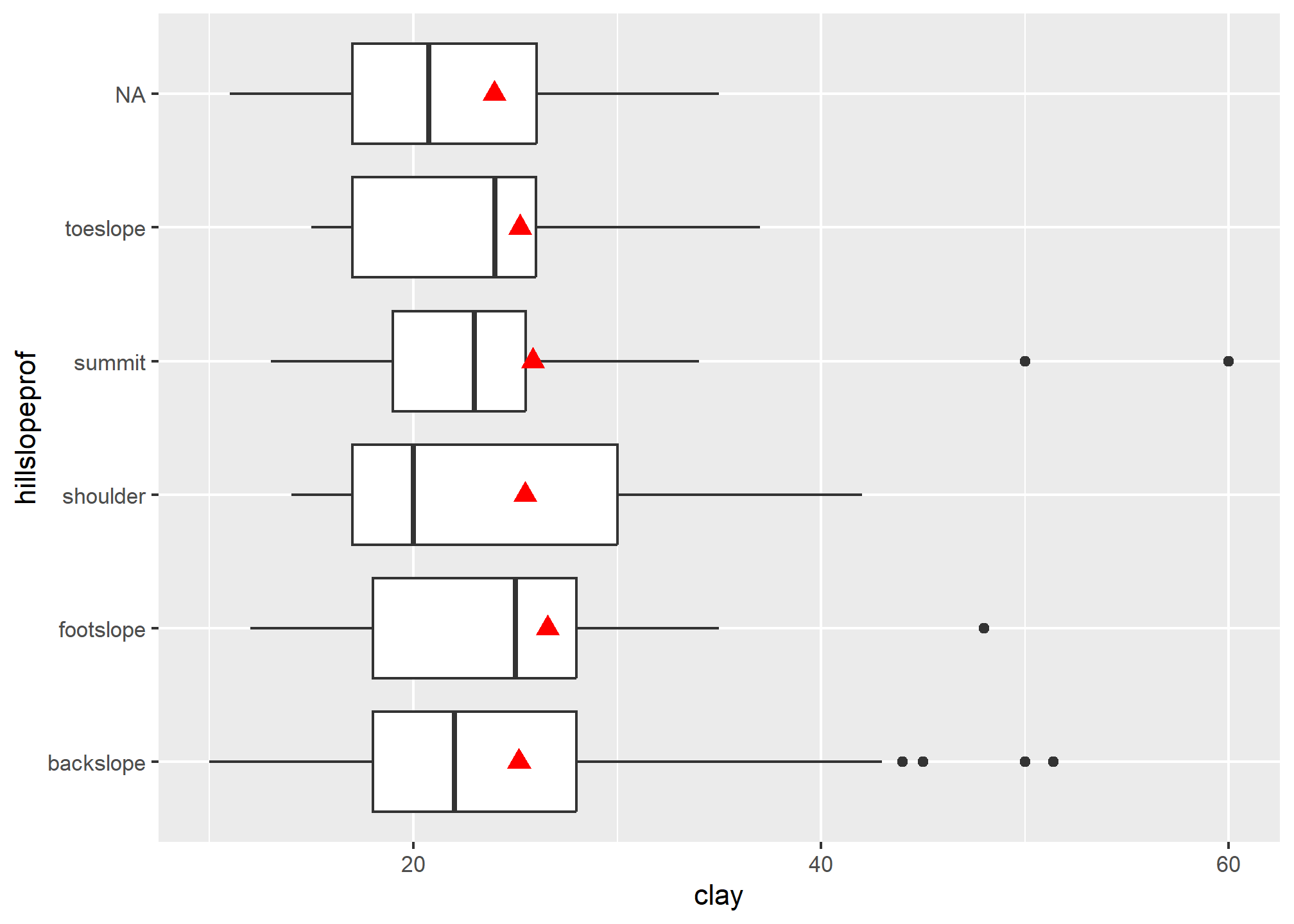

# use site-level columns for profile-specific intervals (e.g. PSCS)
ggplot() +
  stat_depth_weighted(
    loafercreek,
    aes(clay, hillslopeprof),
    na.rm = TRUE,
    from = psctopdepth,
    to = pscbotdepth
  )