Accessing 'Rangeland Analysis Platform' (RAP) Products with R • rapr

library(rapr)    # access RAP products
library(terra)   # spatial data handling

## terra 1.8.93

First, we buffer 1000 meters around a longitude/latitude coordinate (WGS84 decimal degrees) using the {terra} package.

Change the buffering distance to include different extents around a point.

p <- buffer(terra::vect(
  data.frame(x = -105.97133, y = 32.73437),
  geom = c("x", "y"),
  crs = "OGC:CRS84"
), width = 1000)

You can change the coordinates your favorite range spot!

We can interactively inspect the area of interest, for example using terra::plet() {leaflet} map:

terra::plet(p, tiles = c("Esri.WorldImagery", "OpenTopoMap"))

Then we use {rapr} to download the ‘Rangeland Analysis Platform’ “vegetation-biomass” product for 1986 to 2024 using the polygon p to define the area of interest.

rap <- get_rap(
  p,
  product = "vegetation-biomass",
  years = 1986:2024,
  verbose = FALSE
)

Once that’s done, let’s look at the first layer:

plot(rap[[1]], main = names(rap)[1])

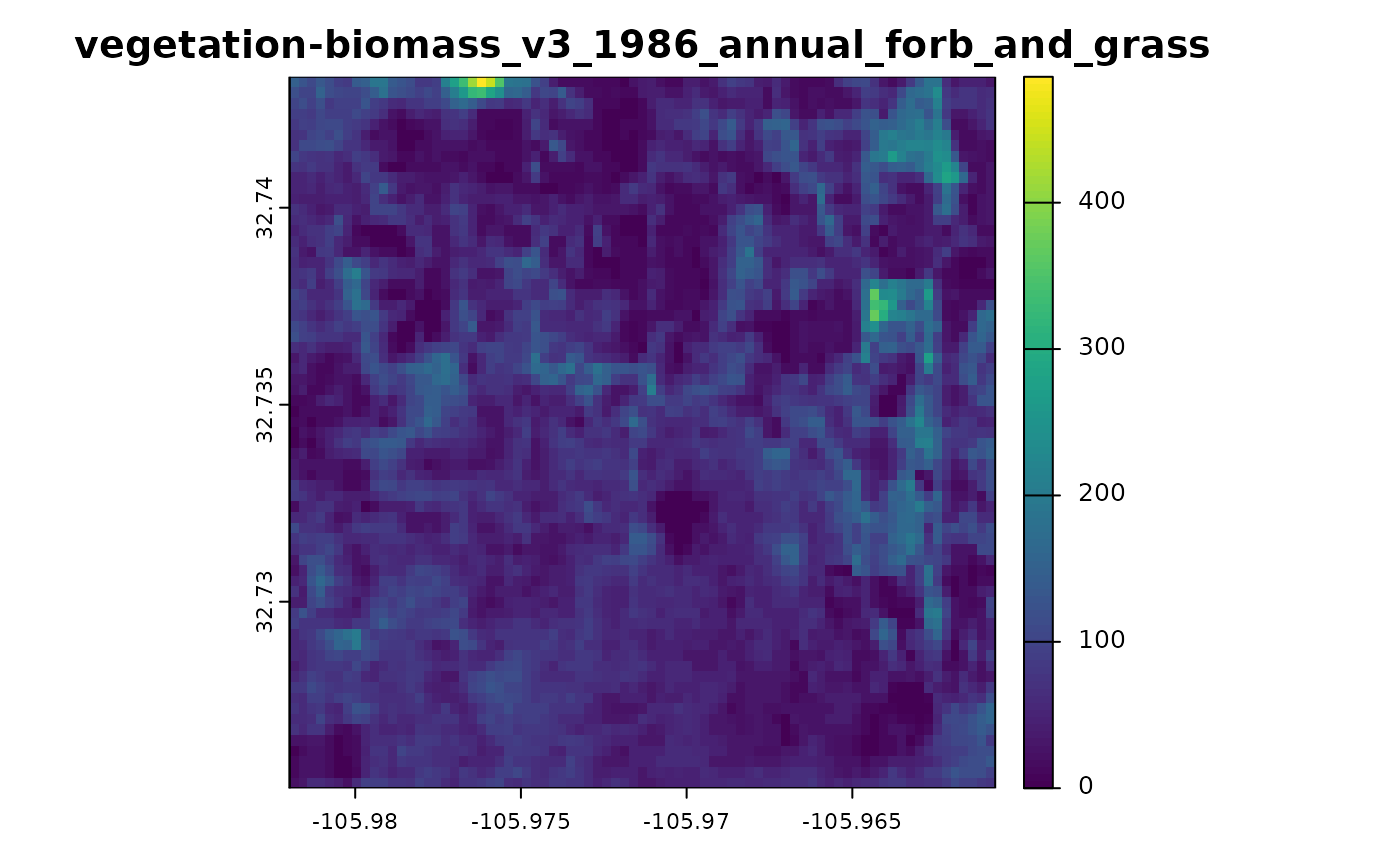
Animated Plots

Now we will select just the "annual forb and grass biomass" layers, iterate over them, and plot. We are symbolizing with a common range of [0,500] pounds per acre so the color scheme is consistent from year to year. We write this iteration into a function called makeplot() and use {gifski} to render an animated GIF file from the R plot graphics output in each year for a total of 39 layers.

makeplot <- function() {
  lapply(grep("annual_forb_and_grass", names(rap)), function(i) {
    terra::plot(
      rap[[i]],
      main = names(rap)[i],
      type = "continuous",
      range = c(0, 500),
      cex.main = TRUE
    )
    terra::plot(
      terra::as.lines(p),
      col = "white",
      add = TRUE
    )
  })
}

Using the {gifski} package save_gif() function we can easily create an animated graphic of the RAP predictions:

try({
  
library(gifski) 
gifski::save_gif(makeplot(), 
                 gif_file = "annual_forb_and_grass_biomass.gif", 
                 delay = 0.5)

})

## [1] "annual_forb_and_grass_biomass.gif"

Tabular data

Finally, we will use {rapr} to download mean fractional vegetation cover values (% cover) from 1995 to 2025, again using the polygon p to define the area of interest.

rap_tab <- get_rap_table(
  p,
  product = "cover",
  years = 1995:2025
)

Once the vegetation cover data has finished downloading, let’s look at the table:

print(rap_tab)

##    year       AFG       PFG       SHR        TRE       LTR      BGR feature
## 1  1995 0.2525703 15.482731  9.150528 0.03005444 11.251535 51.98333       1
## 2  1996 3.2239168 22.719430  5.769740 0.04252105 12.277209 52.71497       1
## 3  1997 1.3700150 21.618796  8.982807 0.56477746 14.824422 49.85788       1
## 4  1998 0.3055703 17.591029 11.156326 0.52369927 11.213395 54.27830       1
## 5  1999 1.0604601 16.598249 10.368510 0.33349172  9.806776 53.82368       1
## 6  2000 3.0121891 20.004445  9.396048 0.32871459  9.391676 53.49902       1
## 7  2001 0.5941018 16.202919 10.505615 0.44086396 12.355832 54.59192       1
## 8  2002 0.1517499 11.489255 10.382267 0.13612410  9.300760 53.61022       1
## 9  2003 0.6772709 15.344910  9.152883 0.11986139  9.308226 58.54672       1
## 10 2004 0.4969863 10.331036  9.178885 0.12477369 10.100490 59.98506       1
## 11 2005 0.6949601  7.714110 10.682500 0.12867424  8.431474 56.23788       1
## 12 2006 2.2794912 21.178261  6.594299 0.05469480  9.680942 56.32850       1
## 13 2007 7.3250414 19.087595  8.061492 0.20420203 13.848843 50.85074       1
## 14 2008 5.9836820 29.407243 12.452279 0.59302345 11.020385 38.26353       1
## 15 2009 2.3985948 19.659387 11.862347 1.52497010 15.655091 43.52256       1
## 16 2010 0.7877624 19.813390 14.963918 0.88433716 12.340159 41.73787       1
## 17 2011 0.2255593 16.938553 11.277027 0.39273733 12.762917 44.54356       1
## 18 2012 0.2476181 13.725517  6.865507 0.06271095 10.640892 50.98776       1
## 19 2013 1.3641084 14.347383  7.364759 0.07581964  8.667634 57.03888       1
## 20 2014 5.2428277 15.010174  6.848346 0.11014021 11.643299 56.44147       1
## 21 2015 2.1831038 12.249271  9.326208 0.21292989 13.002112 55.77812       1
## 22 2016 0.8279138  9.929319 13.454206 0.36809492 10.400814 54.83675       1
## 23 2017 1.2086586  9.834304 13.978861 0.22973842 10.111731 53.61740       1
## 24 2018 0.4815561 11.086233 12.687578 0.09839554  9.661289 51.71096       1
## 25 2019 0.6166654  9.966145 11.527014 0.06754440  8.731150 55.35689       1
## 26 2020 1.2325842  9.554955 13.699356 0.20734685 10.601484 50.77042       1
## 27 2021 2.1373468 12.619353 13.246030 0.27328044  8.868258 50.13520       1
## 28 2022 2.6766667 16.393730 12.602006 0.64226832 11.069478 46.95834       1
## 29 2023 0.7184658 14.582831 13.345551 0.25087657 10.745843 45.28449       1
## 30 2024 0.3039851  7.834614 13.623864 0.22431410  9.926046 49.30078       1
## 31 2025 0.3061008  7.647572 12.380474 0.09271214  9.262576 52.32375       1

and plot mean "PFG" (Perennial Forb and Grass cover) over those 20 years:

plot(rap_tab$year, 
     rap_tab$PFG, 
     xlab="Year", 
     ylab="Perennial Forb and Grass cover (%)", 
     type="l")